Key Strategies for Identifying Plant Bottlenecks
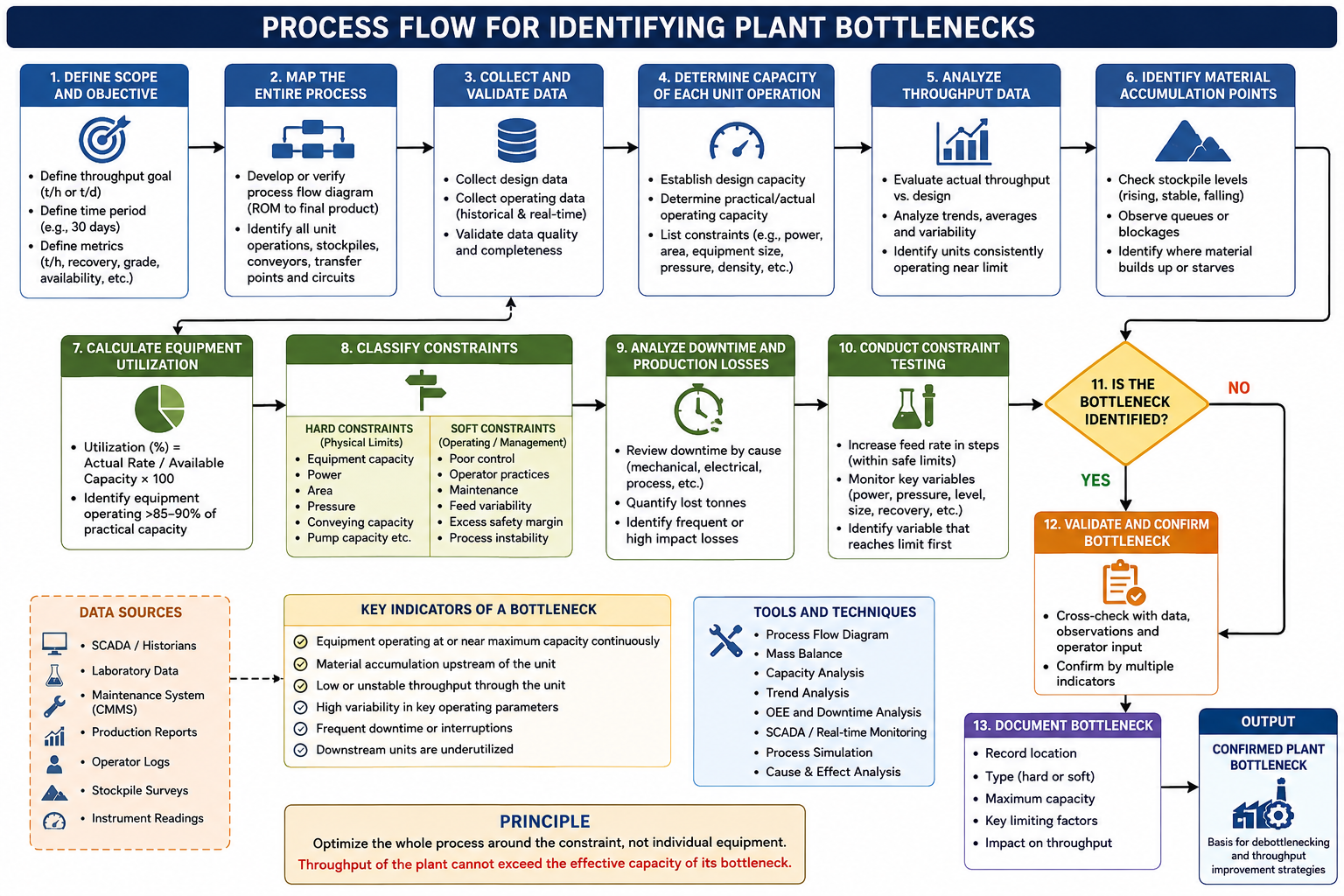
A bottleneck is the process, equipment, or operating constraint that **limits the overall production rate** of the plant.
### 1. Map the Entire Process Flow
Start with a complete process flow diagram from **ROM feed to final product**.
Identify:
* Crushing and screening
* Stockpiles and reclaiming
* Conveyors and transfer points
* Grinding
* Classification
* Flotation, DMS or other separation
* Thickening and filtration
* Product handling
The objective is to understand where material can accumulate, where flow is restricted, and where capacity changes between process stages.
### 2. Determine the Capacity of Each Unit
Operation Establish the **design capacity versus actual operating capacity** for every major piece of equipment.
The bottleneck is often revealed when one unit consistently operates close to its maximum capacity while upstream equipment has spare capacity.
### 3. Analyze Throughput Data
Use historical operating data rather than relying only on design specifications.
Analyze:
* t/h
* tonnes/day
* instantaneous versus average throughput
* operating hours
* equipment loading
* downtime
* production losses
* feed variability
Look for equipment or process areas where throughput repeatedly reaches a ceiling.
### 4. Identify Accumulation Points
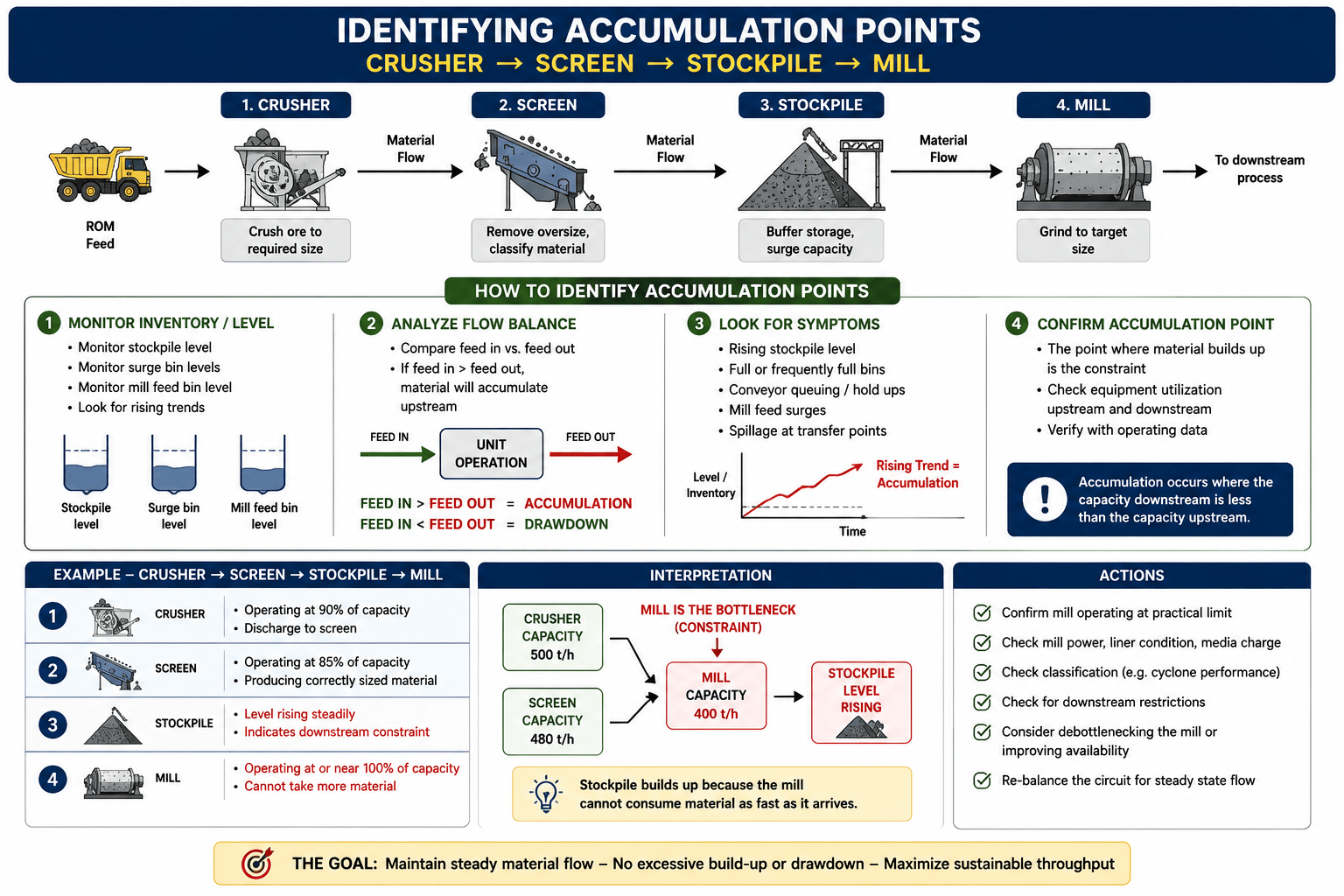
**Material accumulation is one of the strongest indicators of a bottleneck.**
For example: **Crusher → Screen → Stockpile → Mill**
If the stockpile continuously increases, the upstream section may have greater capacity than the downstream mill. Conversely, if the stockpile continuously decreases, the downstream section may have excess capacity relative to the upstream feed system.
### 5. Examine Equipment Utilization
Calculate utilization for critical equipment:
**Utilization (%) = Actual Operating Rate / Available Capacity × 100**
Equipment operating continuously at or near its practical limit should be investigated as a potential bottleneck.
However, **high utilization alone does not prove that the equipment is the bottleneck**. The interaction between process units must also be considered.
### 6. Separate Hard and Soft Bottlenecks
This is particularly important. **Hard bottlenecks** are physical limitations such as:
* Crusher capacity
* Mill power
* Conveyor capacity
* Pump capacity
* Screen area
* Cyclone capacity
* Thickener area
**Soft bottlenecks** are operating or management constraints such as:
* Conservative operating practices
* Poor control strategies
* Excessive safety margins
* Operator intervention
* Poor maintenance
* Feed variability
* Inadequate process control
A plant may have significant **hidden capacity** because of a soft bottleneck rather than a physical equipment limitation.
### 7. Analyze Downtime and Production Losses
Perform a **production-loss analysis** and categorize lost tonnes into:
* Mechanical failures
* Electrical failures
* Process interruptions
* Blockages
* Start-up/shutdown losses
* Feed shortages
* Maintenance
* Operator-related delays
* Product quality constraints
A machine that has sufficient capacity but frequently stops may be a bigger throughput constraint than a machine operating continuously near its design capacity.
### 8. Conduct Constraint Testing Carefully
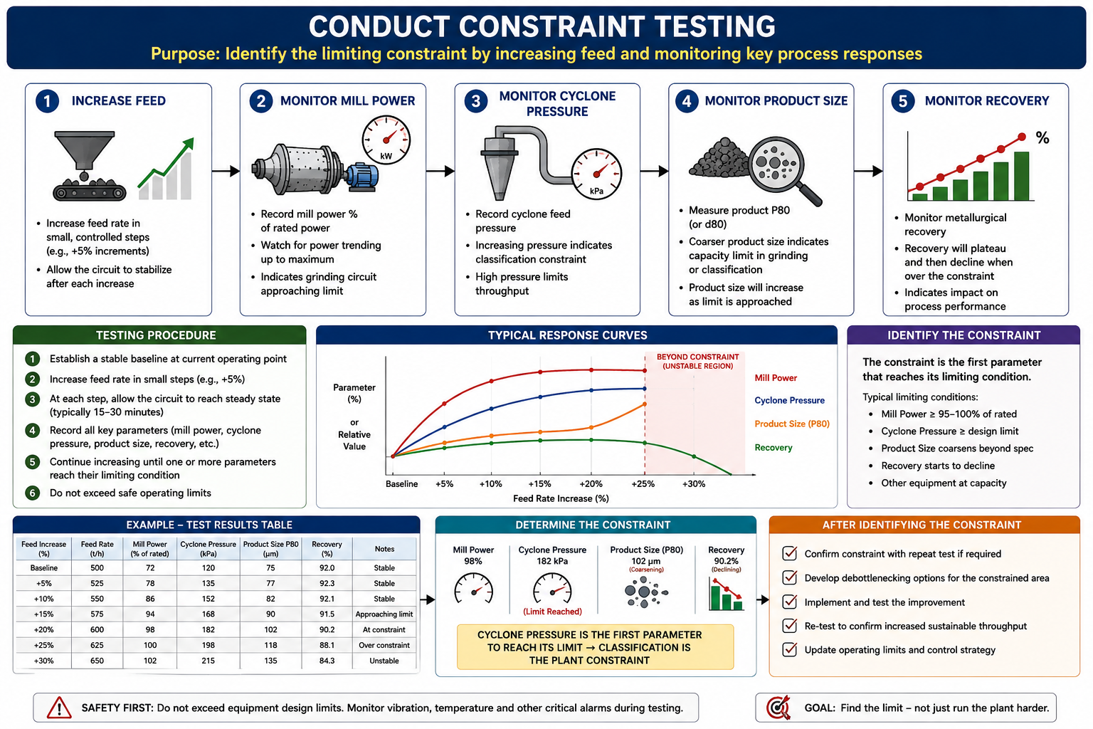
increase feed rate while monitoring critical variables.
For example:
**Increase feed → Monitor mill power → Monitor cyclone pressure → Monitor product size → Monitor recovery**
This helps determine which variable reaches its operating limit first. Constraint testing should be conducted within **equipment, process, safety and environmental operating limits**.
### 9. Use Mass Balance and Process Simulation
A plant-wide mass balance can identify inconsistencies and capacity restrictions.
Process simulation can then be used to test scenarios such as:
* +5% feed rate
* +10% feed rate
* Increased crusher capacity
* Increased mill power
* Improved screening efficiency
* Reduced circulating load
* Additional flotation capacity
This helps determine whether increasing one piece of equipment will actually increase **overall plant throughput**.
### 10. Use Real-Time Process Data
Modern plants can use SCADA, historians, APC and analytics to identify bottlenecks dynamically.
Monitor variables such as:
**Feed rate → Equipment loading → Power → Pressure → Density → Level → Particle size → Recovery**
This allows the plant to distinguish between a **permanent bottleneck** and a **temporary operating constraint**.
--- ## The Bottleneck Identification Process
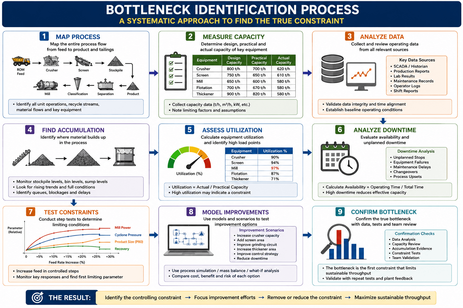
A practical approach is:
**1. Map Process → 2. Measure Capacity → 3. Analyze Data → 4. Find Accumulation → 5. Assess Utilization → 6. Analyze Downtime → 7. Test Constraints → 8. Model Improvements → 9. Confirm Bottleneck**
### Most Important Principle
> **Do not optimize individual equipment in isolation.
Optimize the entire process around the system constraint.
** For example, increasing crusher capacity from **500 to 600 t/h** will not increase plant production if the grinding circuit can only process **450 t/h**. In that situation, the **grinding circuit—not the crusher—is the effective plant bottleneck**.
This systems approach is particularly important when developing a **“Maximizing Plant Throughput”** article because it leads naturally into the next sections: **bottleneck analysis → debottlenecking → process optimization → advanced process control → maintenance → continuous improvement**.
Role and Importance of Mapping the Entire Process Flow
**Mapping the entire process flow** is a critical first step in identifying plant bottlenecks and maximizing mineral processing plant throughput. It provides a complete picture of how ore, water, reagents, energy and information move through the plant—from **ROM feed to final product and tailings**.
### 1. Provides a Complete View of the Plant
A process flow map shows all major unit operations and their connections, including: **ROM → Crushing → Screening → Stockpile → Grinding → Classification → Separation → Thickening → Filtration → Product** It prevents individual equipment from being analyzed in isolation.
### 2. Identifies Potential Bottlenecks
The flow diagram makes it easier to identify areas where capacity may be restricted, such as:
* Crushers operating at maximum capacity
* Screens with insufficient capacity
* Conveyor restrictions
* Mill power limitations
* Cyclone capacity constraints
* Flotation residence-time limitations
* DMS capacity restrictions
* Thickener or filtration limitations
The key question is:
> **Where can the flow of material be restricted, delayed or interrupted?**
### 3. Establishes the Relationship Between Unit Operations
Mineral processing plants are **interdependent systems**. Increasing the capacity of one unit does not necessarily increase overall plant throughput. For example: **Crusher: 600 t/h → Mill: 450 t/h → Flotation: 500 t/h** The grinding circuit becomes the effective bottleneck because the plant cannot continuously process more than approximately **450 t/h through the constrained circuit**.
### 4. Identifies Material Accumulation Points
Mapping the process allows operators to track where material accumulates.
Typical indicators include:
* Increasing stockpile levels
* Full surge bins
* Conveyor queues
* High mill feed bins
* Increasing circulating loads
* Thickener inventory increases Accumulation can indicate that an **upstream operation has more capacity than the downstream operation**.
### 5. Supports Mass-Balance Analysis
A process flow diagram provides the framework for establishing a plant-wide **mass balance**. Important streams include:
* Feed
* Concentrate/product
* Middlings
* Tailings
* Recycle streams
* Water
* Reagent additions
Mass balance helps identify unexplained losses, abnormal recirculation and capacity constraints.
### 6. Highlights Recycle and Recirculating Loads
Some circuits contain significant internal recycling.
For example: **Mill → Cyclone → Oversize → Mill** If the circulating load becomes excessive, the grinding circuit may become constrained even though the nominal mill capacity appears adequate.
Mapping these recycle streams is therefore essential when investigating bottlenecks.
### 7. Identifies Dependencies Between Equipment
The process map shows which equipment depends on other equipment. For example: **Crusher → Screen → Conveyor → Stockpile → Reclaimer → Mill**
A failure in the conveyor can effectively stop the mill even though the mill itself is fully operational. This helps distinguish between **equipment bottlenecks and system bottlenecks**.
### 8. Provides a Basis for Data Collection
Once the process has been mapped, specific measurements can be assigned to each stage:
### 9. Helps Identify Hidden Constraints
Not all bottlenecks are obvious physical capacity limitations.
A process map can reveal **soft constraints**, such as: * Poor control strategy
* Inadequate surge capacity
* Poor stockpile management
* Feed variability
* Operator practices
* Maintenance practices
* Poor instrumentation
* Unstable process conditions
These constraints may represent significant **hidden production capacity**.
### 10. Establishes a Baseline for Debottlenecking
Once the entire process has been mapped, the plant team can establish:
**Current capacity → Constraint → Bottleneck → Improvement opportunity → Expected throughput increase** This creates a structured basis for evaluating potential investments and operational improvements.
--- ### Key Principle
> **You cannot reliably identify a plant bottleneck without understanding the complete process flow and the interaction between its individual unit operations.** Mapping the process therefore provides the **foundation for capacity analysis, mass balancing, bottleneck identification, debottlenecking and throughput optimization**.
Methods for Mapping the Entire Process Flow
There are several methods available for mapping the complete process flow of a mineral processing plant. The best approach is usually to **combine several methods**, because a single flowsheet rarely captures the actual operating conditions, material movements, bottlenecks and control constraints.
### 1. Process Flow Diagram (PFD)
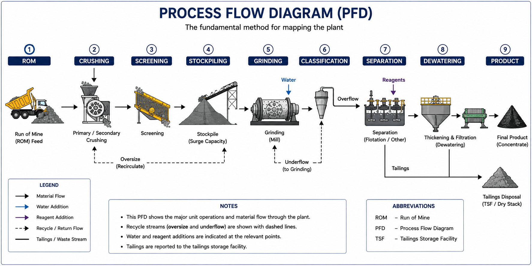
The **Process Flow Diagram** is the fundamental method for mapping the plant. It shows: **ROM → Crushing → Screening → Stockpiling → Grinding → Classification → Separation → Dewatering → Product**
A PFD normally identifies:
* Major equipment
* Material streams
* Feed and product flows
* Recycle streams
* Water additions
* Reagent additions
* Major operating parameters
**Best for:** Establishing the overall plant structure.
--- ### 2. Piping and Instrumentation Diagram (P&ID)
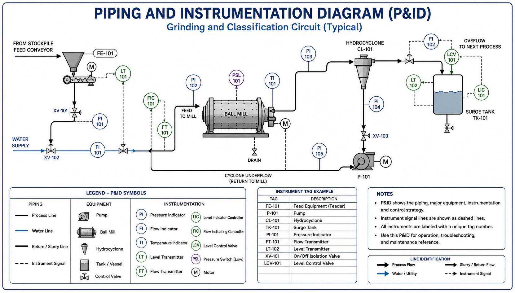
A **P&ID** provides a much more detailed representation of the process. It includes:
* Pumps
* Valves
* Pipelines
* Instruments
* Control loops
* Flow meters
* Pressure transmitters
* Level instruments
* Density meters
* Control valves
**Best for:** Understanding instrumentation, control systems and process constraints.
--- ### 3. Material Flow Mapping
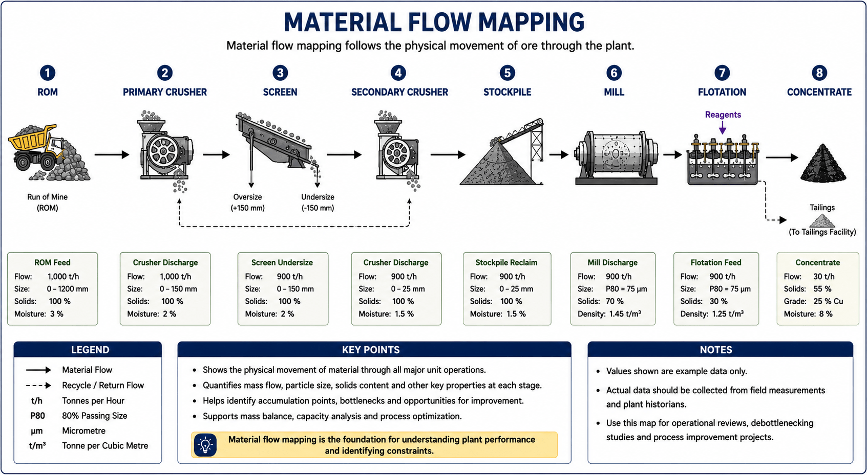
Material flow mapping follows the physical movement of ore through the plant.
For example: **ROM → Primary Crusher → Screen → Secondary Crusher → Stockpile → Mill → Flotation → Concentrate** At each stage, determine: **Feed rate → Product rate → Recirculating load → Losses**
**Best for:** Identifying accumulation points, flow restrictions and material bottlenecks.
--- ### 4. Mass-Balance Mapping
Mass-balance mapping quantifies the material entering and leaving each process stage.
For example:
**Feed = Product + Tailings + Losses ± Inventory Change**
It can be applied to:
* Total solids
* Water
* Valuable minerals
* Gangue
* Concentrate
* Tailings
**Best for:** Identifying inconsistencies, losses, recycle loads and capacity constraints.
--- ### 5. Value Stream Mapping (VSM)
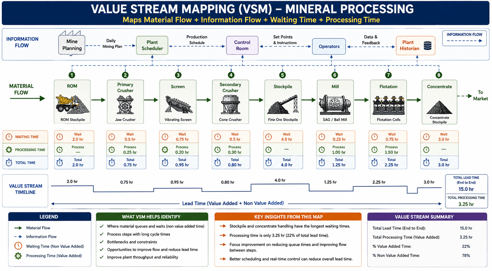
Value Stream Mapping originates from Lean manufacturing but can be adapted to mineral processing.
It maps: **Material Flow + Information Flow + Waiting Time + Processing Time**
It can identify:
* Waiting
* Queuing
* Excess inventory
* Unnecessary handling
* Delays
* Process interruptions
**Best for:** Identifying operational inefficiencies beyond equipment capacity.
--- ### 6. Equipment Capacity Mapping
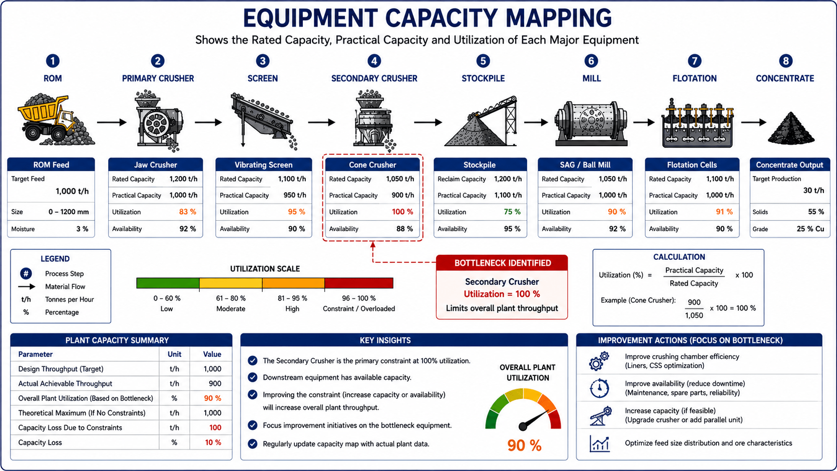
Create a capacity map for every major unit operation.
| Unit Operation | Design Capacity | Practical Capacity | Actual Rate | Utilization | | --------------- | --------------: | -----------------: | ----------: | ----------: | | Primary crusher | 800 t/h | 700 t/h | 650 t/h | 93% | | Screening | 750 t/h | 680 t/h | 650 t/h | 96% | | Grinding | 650 t/h | 600 t/h | 590 t/h | 98% | | Flotation | 700 t/h | 670 t/h | 590 t/h | 88% |
This makes potential constraints much easier to identify.
**Best for:** Bottleneck and debottlenecking studies.
--- ### 7. Digital Process Mapping
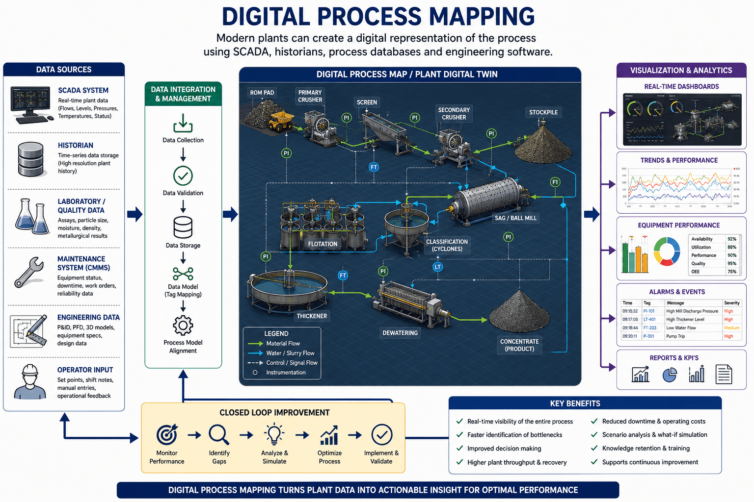
Modern plants can create a **digital representation of the process** using SCADA, historians, process databases and engineering software.
Real-time data can be linked to:
* Equipment
* Process streams
* Sensors
* Control loops
* Production KPIs
The result is a dynamic process map rather than a static drawing.
**Best for:** Real-time monitoring and operational optimization.
--- ### 8. Process Simulation
Process simulation models the plant mathematically and allows different operating scenarios to be tested. For example: **Current feed = 500 t/h** Simulation scenarios: * 550 t/h * 600 t/h * 650 t/h The model can determine where constraints occur as throughput increases.
**Best for:** Predicting bottlenecks before making capital investments.
--- ### 9. SCADA/Historian-Based Mapping
Historical and real-time SCADA data can be used to map how the plant actually operates.
Typical variables include:
* Feed rate
* Flow
* Density
* Pressure
* Level
* Power
* Temperature
* Particle size
* Equipment status
Trend analysis can reveal recurring throughput restrictions that may not be obvious from engineering drawings.
**Best for:** Identifying dynamic and intermittent bottlenecks.
--- ### 10. Physical Plant Walkdown
A physical **plant walkdown** is extremely valuable.
Engineers and operators physically follow the material path through the plant and verify:
**What the drawing says → What the plant actually does**
Look for:
* Blockages
* Spillage
* Material accumulation
* Bypasses
* Temporary modifications
* Unused equipment
* Restricted chutes
* Poor transfer points
* Equipment accessibility problems
**Best for:** Validating the process map against actual plant conditions.
--- ### 11. Drone, Laser Scanning and 3D Mapping
For large or complex plants, technologies such as:
* **3D laser scanning**
* **LiDAR**
* **Drone surveys**
* **Photogrammetry**
* **3D plant modelling** can create accurate digital representations of the plant.
These are particularly useful where **as-built drawings are incomplete or outdated**. **Best for:** Brownfield plants, expansion projects and physical layout analysis.
--- ### 12. Process Mining and Data Analytics
Process mining uses historical operational data to reconstruct how the plant actually behaves. It can identify:
* Process sequences
* Delays
* Repeated interruptions
* Equipment interactions
* Operating patterns
* Abnormal process states
This is particularly useful for complex automated plants.
**Best for:** Finding hidden operational bottlenecks and recurring production losses.
--- ## Recommended Approach
For a mineral processing plant, I recommend combining the methods rather than relying on one.
### **Integrated Process Mapping Approach**
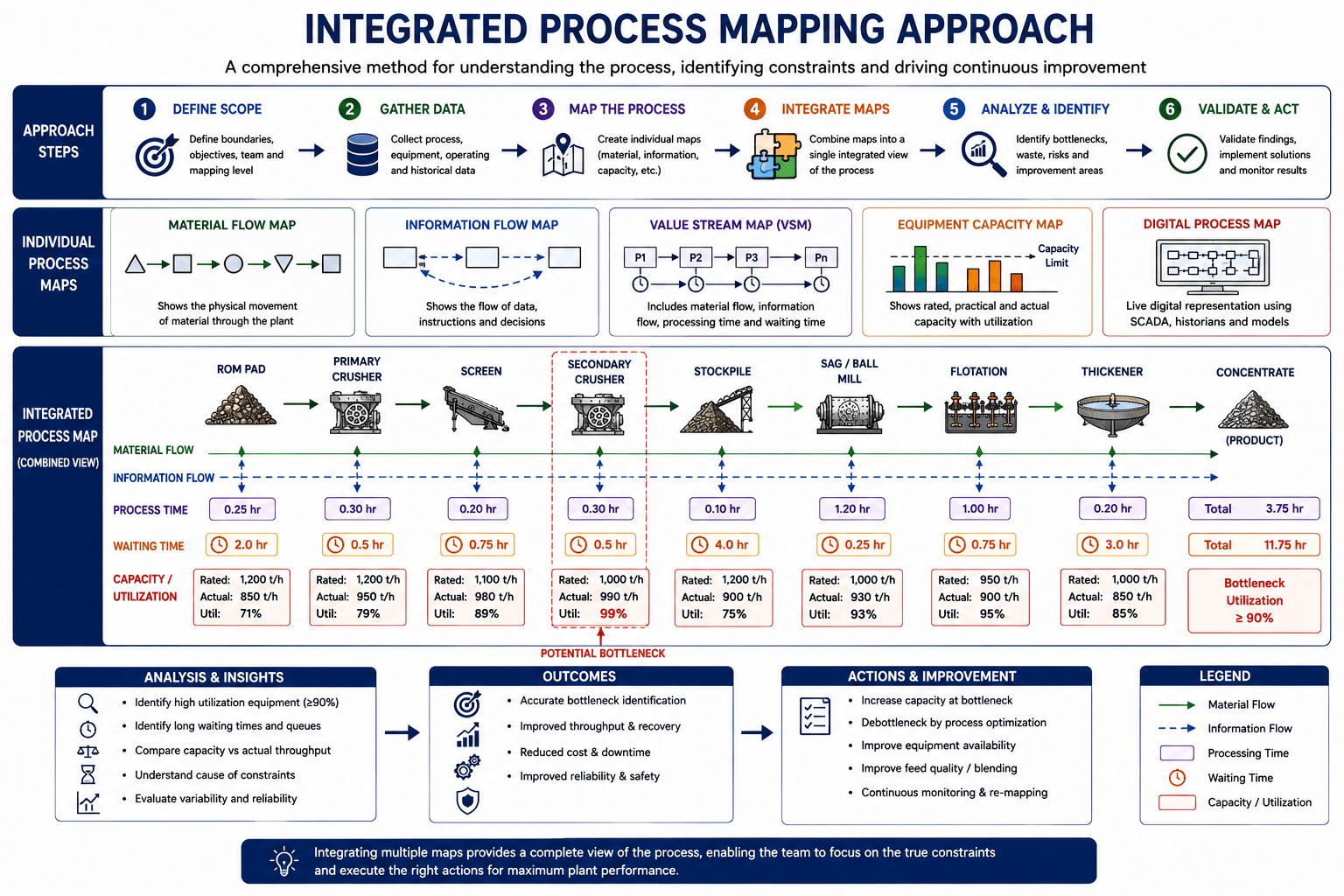
**1. Existing PFD/P&ID** ↓ **2. Physical Plant Walkdown** ↓ **3. Equipment Capacity Mapping** ↓ **4. Material Flow & Mass Balance** ↓ **5. SCADA/Historian Data Analysis** ↓ **6. Bottleneck & Constraint Analysis** ↓ **7. Process Simulation** ↓ **8. Validate Against Actual Plant Performance** ↓
### **9. Confirm Plant Bottleneck**
### Key takeaway The **PFD tells you how the plant is supposed to operate**, while the **plant walkdown and operating data tell you how it actually operates**.
Combining these with mass balance, capacity analysis and simulation provides a much more reliable basis for identifying the **true plant bottleneck** and determining where throughput improvements will deliver the greatest benefit.
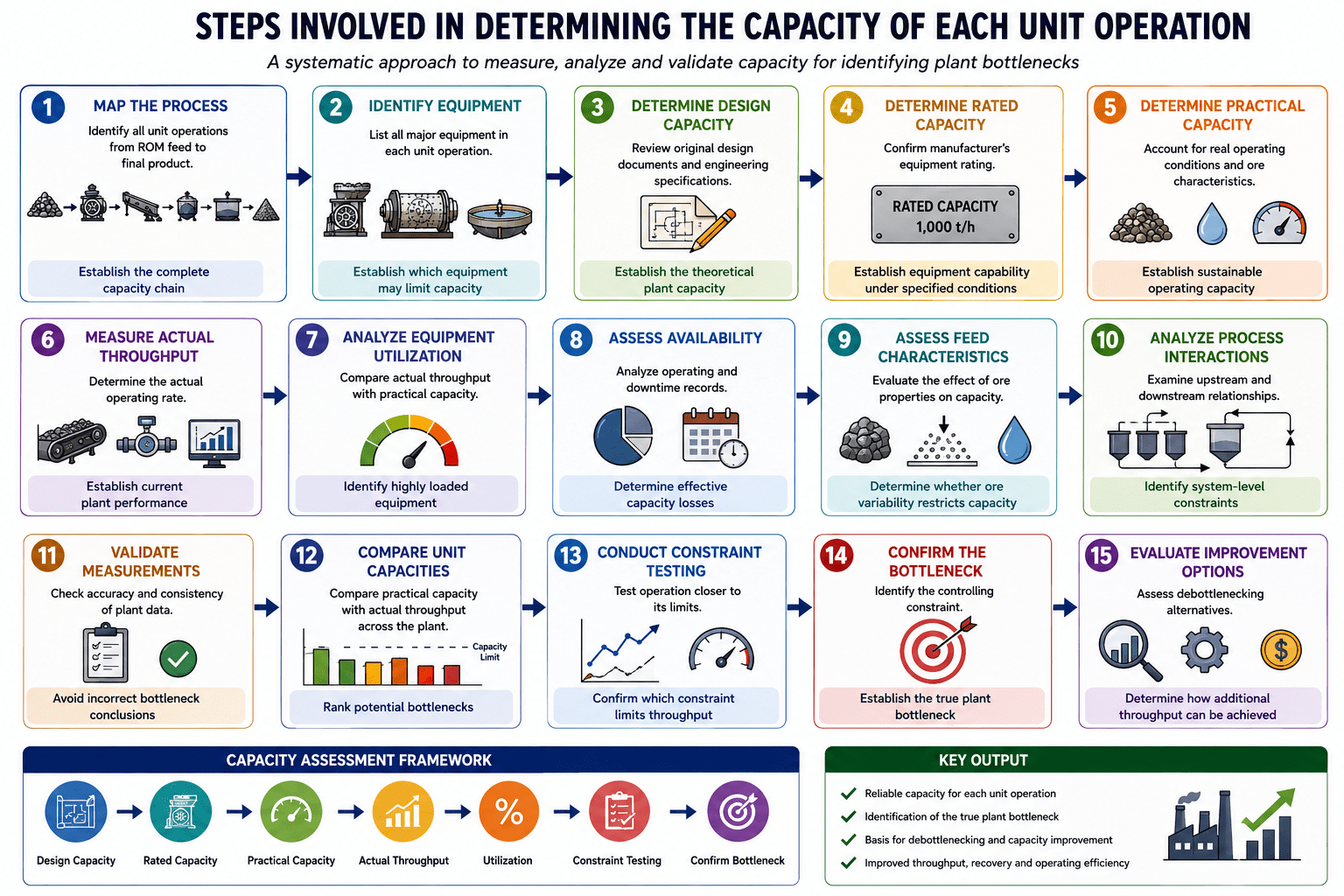
Determining the Capacity of Each Unit Operation
Determining the capacity of each unit operation is a critical step in **identifying plant bottlenecks**.
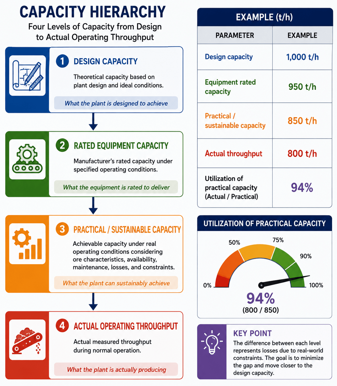
The objective is to establish the difference between the **design capacity, rated capacity, practical operating capacity and actual throughput** of each major unit operation.
### 1. Steps Involved
### 2. Capacity Hierarchy
It is useful to distinguish four different capacity levels: **Design Capacity** ↓ **Rated Equipment Capacity** ↓ **Practical/Sustainable Capacity** ↓ **Actual Operating Throughput**
### 3. Important Factors to Consider
#### Equipment Characteristics
* Equipment size and configuration
* Motor power
* Crusher chamber dimensions
* Mill volume and installed power
* Screen area and aperture
* Pump capacity
* Conveyor width and speed
* Thickener diameter
#### Ore Characteristics
* Feed size distribution
* Ore hardness
* Abrasiveness
* Moisture content
* Bulk density
* Clay content
* Mineralogy
* Liberation characteristics
#### Operating Conditions
* Feed rate
* Equipment loading
* Mill density
* Cyclone pressure
* Screen loading
* Crusher CSS
* Pump operating point
* Residence time
* Circulating load
#### Availability and Reliability
* Mechanical failures
* Electrical failures
* Planned maintenance
* Unplanned downtime
* Blockages
* Start-up and shutdown losses
Challenges in Determining Unit Operation Capacity
A piece of equipment may be rated at 1,000 t/h, but actual sustainable performance may only be 800–900 t/h because of ore characteristics or operating constraints. Therefore, relying solely on manufacturer's specifications can result in an incorrect bottleneck assessment.
2. Variable Ore Characteristics
Ore properties can change significantly during the life of a mine.
For example: Harder ore → Higher power requirement → Lower mill throughput → Grinding becomes the bottleneck Similarly: Wet/clayey ore → Screen blinding → Reduced screening capacity → Crusher circuit constraint
3. Interdependence Between Equipment
Unit operations cannot always be assessed independently.
For example: Crusher → Screen → Stockpile → Mill
A crusher may have spare capacity while the screen is limiting the flow. Increasing crusher capacity would therefore provide little or no increase in plant throughput.
4. Measuring Actual Flow Can Be Difficult
Reliable throughput measurements are essential, but instruments can suffer from: Calibration errors Poor installation Sensor drift Material build-up Belt-scale inaccuracies Density measurement errors Sampling errors Poor-quality data can lead to an incorrect bottleneck diagnosis.
5. Intermittent Bottlenecks
Some bottlenecks occur only under particular conditions. For example, a mill may normally process 900 t/h but drop to 700 t/h when: Hard ore is encountered Feed moisture increases Mill power reaches its limit Cyclone pressure becomes unstable This means that average throughput may hide a dynamic bottleneck.
6. Recycle and Circulating Loads
Internal recycle streams can significantly affect capacity.
For example: Mill → Cyclone → Oversize → Mill An increase in circulating load can consume available mill capacity even though fresh ore feed remains unchanged.
7. Downtime Masks Capacity
An equipment item may appear to have adequate capacity when it is actually losing significant production through frequent stoppages.
For this reason, capacity analysis should consider both:
Capacity × Availability = Effective Capacity
8. Lack of Reliable Historical Data
Older plants may have: Incomplete SCADA records Missing production data Manual measurements Poorly calibrated instruments Changes in equipment configuration Outdated process documentation This makes it difficult to establish a reliable capacity baseline.
9. Temporary Operating Constraints
An apparent bottleneck may actually be caused by a temporary condition such as: Equipment under maintenance Temporary ore characteristics Low stockpile inventory Water shortage Reagent shortage Downstream equipment outage It is therefore important to distinguish between a temporary constraint and a persistent bottleneck.
10. Safety and Environmental Constraints
The maximum sustainable capacity may be below the theoretical equipment capacity because of:
Dust emissions Noise Tailings capacity Water availability Structural limitations Equipment safety limits Environmental operating conditions
These constraints must be included in the capacity assessment. Capacity Assessment for Bottleneck Identification
A useful approach is to create a Unit Operation Capacity Matrix:
Unit Operation Rated Capacity Practical Capacity Actual Throughput Utilization Potential Constraint Primary Crusher 1,200 t/h 1,000 t/h 850 t/h 85% Low Screen 1,100 t/h 900 t/h 850 t/h 94% High Secondary Crusher 1,000 t/h 850 t/h 840 t/h 99% Critical Stockpile 1,200 t/h 1,100 t/h 850 t/h 77% Low Mill 1,000 t/h 900 t/h 850 t/h 94% High Flotation 950 t/h 900 t/h 850 t/h 94% High Thickener 1,000 t/h 950 t/h 850 t/h 89% Moderate The secondary crusher would be the first unit to investigate because it is operating closest to its practical capacity.
Key Principle
The bottleneck is not necessarily the equipment with the lowest design capacity; it is the constraint that prevents the entire plant from sustainably processing more material.
Therefore, determining unit-operation capacity should combine engineering specifications, actual operating data, ore characteristics, equipment availability, process interactions and controlled performance testing. This provides a much more reliable basis for identifying and ultimately removing the plant bottleneck.
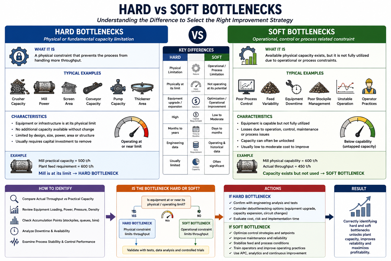
Separating Hard and Soft Bottlenecks in Mineral Processingd
1. Hard Bottlenecks
A hard bottleneck is a physical or fundamental capacity limitation that prevents a process from handling additional throughput.
Typical examples include:
- Crusher maximum capacity
- Mill installed power
- Screen area Conveyor capacity
- Pump capacity
- Cyclone capacity
- Flotation cell volume DMS plant capacity
- Thickener area Filter capacity Pipeline capacity
- Structural or physical limitations
For example:
Mill practical capacity = 500 t/h Plant feed requirement = 600 t/h If the mill is already operating at its practical limit, the grinding circuit represents a hard bottleneck.
2. Soft Bottlenecks A soft bottleneck occurs when available physical capacity is not fully utilized because of operating, control, maintenance or process-related constraints.
Examples include:
- Poor process control Inadequate instrumentation
- Poor operator practices Feed variability
- Poor stockpile management
- Excessive equipment downtime
- Conservative operating limits
- Poor maintenance practices Inefficient control strategies
- Unstable process conditions
- Poor material handling Inadequate surge capacity
- Suboptimal operating setpoints
For example:
A mill may be physically capable of processing 600 t/h, but poor feed control and unstable cyclone operation restrict actual throughput to 500 t/h. This represents a potential soft bottleneck.
Hard vs Soft Bottlenecks
Identifying the Difference
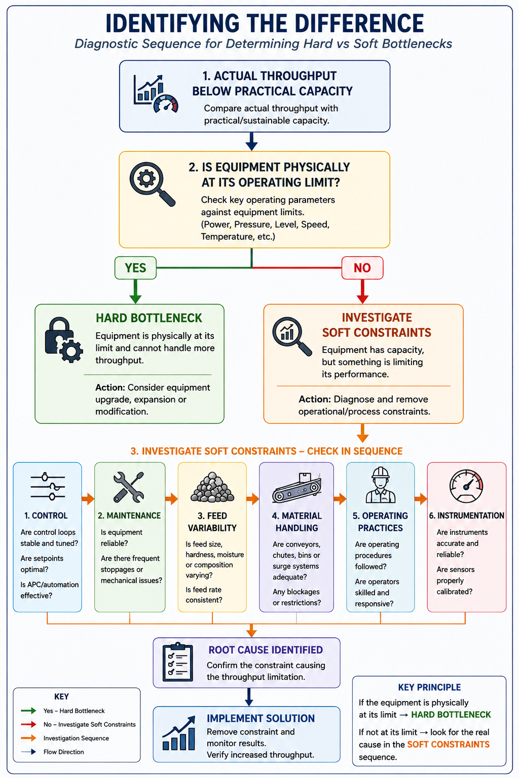
Why the Distinction Matters
For example: If a grinding circuit is processing 450 t/h because the mill has reached its power limit, increasing mill capacity may be necessary.
But: If the mill is physically capable of 550 t/h but is operating at 450 t/h because of unstable feed density and poor cyclone control, improving process control may unlock the additional 100 t/h without major capital expenditure. Key Principle Before investing in additional equipment, determine whether the bottleneck is genuinely physical or whether existing capacity is being lost through operational, control, maintenance or process constraints.
This approach is particularly valuable for debottlenecking studies, because removing a soft bottleneck can often provide a faster and lower-cost throughput improvement than expanding equipment capacity.